Asian Journal of Information Technology
Automatic Assessment for the Detection of Knee Effusion using Magnetic Resource Imaging
Authors : Aamir Yousuf Bhat and A. Suhasini
Abstract: Effusion of the knee joint is possibly related to osteoarthritis erupt and is a significant marker of remedial reaction. The investigation is planned for creating and approving a computerized framework dependent on MR imaging for the measurement of joint effusion. The occurrence of knee effusion requires an extensive differential determination and an orderly symptomatic approach. Yearning of the knee effusion is a fundamentally demonstrative and restorative intercession in numerous rheumatologic diseases. The clinical investigation has traditionally included tests counting the patella tap. The precision of these tests for identifying the effusion and measure is not well set up. MR imaging is considered superior for recognizable proof and evaluation of knee effusion. The amount of effusion present in the joint was recorded and MRI criteria for the detection of knee effusion were assessed. The fat cushion division sign was the foremost exact marker of liquid as little as 1-2 mLwas recognized. Axial view of MRI images was used in accessing the knee effusion. The classifier was superior both in terms of time efficiency and classification performance to classifier regularly used on the basis of iterative learning. In this paper we have used two features namely watershed Segmentation and 2-D Gabor Filter. The extracted features from MRI image are given to the classifiers namely Random Forest, Multi Linear BPNN and Adaboost SVM. The random forest classifier was good when comparing with the other two classifier and achieves the good accuracy rate of 92.12%. Finally, the classifier was prevalent both in time adequacy and order execution to the routinely used classifiers dependent on iterative learning.
How to cite this article:
Aamir Yousuf Bhat and A. Suhasini, 2020. Automatic Assessment for the Detection of Knee Effusion using Magnetic Resource Imaging. Asian Journal of Information Technology, 19: 70-81.
INTRODUCTION
A joint effusion is an abnormal fluid accumulation in or around the knee joint. It is usually caused by infection, injury and arthritis. Knee is the most affected joint by effusion, although, it can occur in ankle, shoulder and hip. There is more evidence that there is synovial inflammation. It plays an important role in OA pathogenesis of the knee. Synovial inflammation could be displayed as synovial membrane. MRI is the most common visualization method used to evaluate the presence and intensity of synovial inflammation. Thickening of the synovial membrane and joint effusion as determined by MRI are often measured together as a whole with the term effusion synovitis as a replaced for synovial inflammation. Joint effusion is often associated with joint disorders. In OA, effusion is an important factor epidemic markers and quantification. This can be useful as a measure of treatment results. The most common method used to measure joint effusion. The main weakness of this method; however, besides being invasive and something that is painful, that you cannot often predict[1]. There is a certain sum of synovial fluid interior of any joint especially in expansive joint such as knee joint. The occurrence of normal amount of synovial fluid cannot be identified by clinical examination as well as by Ultrasound but can be recognized by MRI[2]. For the development of the knee joint synovial liquid is secreted by type B cells of synovial membrane. Synovial fluid moves into the cartilage when a joint is on resting and moves out of the joint space, when the joint is dynamic, especially weight bearing. Synovial fluid incorporates hyaluronic corrosive (HA) lubricin (PRG4), surface-active Phospholipids (SAPL) proteinase and collagenases. Type A is phagocytic cells which evacuates the wear and tear debris from the synovial fluid. HA and PRG4 increment the consistency and flexibility of articular cartilages and grease up the surface between synovium and cartilage.
The characteristics history of MRI detected effusion synovitis in older subjects has not yet been described. It is not known if the knee has structural abnormalities including cartilage defects, reduced cartilage volume, meniscal lesions and bone marrow lesions to produce effusion synovitis. Joint effusion can be distinguished visually from synovitis utilizing contrast enhanced MRI after intravenous gadolinium infusion but method is most commonly utilized for investigation, since of potential side effects and high costs. Knee effusion can be classified as traumatic and non-traumatic. Non-traumatic etiologies incorporate degenerative joint pain, inflammatory arthritis, contamination, precious stone testimony and tumour[3]. There is obvious reason for knee effusion in case of fiery, irresistible, crystal deposition inflection and tumour case. The fore most common reason for degenerative joint pain is overuse repetitive push and dynamic life style. The exact cause of primary OA is still questionable. There is a decrease in the concentration of HA and SAPL in synovial fluid from primary OA patients by the obscure component[4].
During the recent years imperative advances has been made for the improvement of MRI innovation. Strategies have been created to assess quantitatively or semi-quantitatively the structural change that happens within the joint tissues incorporating the cartilage, synovial layer, menisci, subchondral bone during OA[5]. The knee effusion may be common findings in patients with knee problems, although, patients may or may note that his knee is swollen. The clinical tests for identification of knee effusion routinely utilized at present time are patella tap test, fluid test and fluctuation test. The occurrence of knee effusion can be affirmed by MRI, USG, circumferential estimation utilizing a measure tape comparing the estimate of the both knees and volumetry utilizing water uprooting as a cruel to identify limb volume[6]. For the identification of large amount of effusion patella tap and cross change tests are used and for the identification of small amount of effusion, fluid shift tests are utilized.
MATERIALS AND METHODS
Dataset: The dataset used for the experiment are obtained from various clinical centres and hospitals. The dataset compromises the information of 250 patients with 40-60 years of ages which has MRI measurement at base line and follows up. MRI was taken on 1.5-T whole body scanner. The MRI examination compromised of two sequences in axial planes without patient repositioning. T2 weighted gradient echo true fast imaging with steady state precision sequence (T2 true FISP, TR/TE I 6/3 msec, ST/SS, 3/0 mm; FOV, 160 mm, FA, 90°; NEX, 2; matrix, 320×320 pixel; reconstructed image, 320×320 pixel; voxel size, 0.5×0.5×3 mm3) and T1 weighted in phase, out phase gradient echo (GRF) sequence (in TR/TF, 450/2.6 msec; out-TR/TF, 450 msec; 6.4 msec; ST/SS, 3/0 mm, FOV, 180×144 mm; FA, 70°; NEX, 1; matrix 320×256 pixel; reconstructed image, 640×512 pixel and voxel size 0.28×0.28×3 mm3) (Fig. 1 and 2).
Preprocessing: The pre-processing of pictures commonly includes evacuating low frequency background noise, normalizing the intensity of the indidual particles pictures, expelling or improving information pictures earlier to computational processing. The goal of pre-processing is an improvement in the picture information that smoother undesirable mutilations or improves e few picture features for further processing. Four classifications of picture pre-processing strategies concurring to the measure of the pixel neighborhood that is utilized for the calculations of unused pixel brightness: pixel brightness transformation, pre-processing techniques that utilize a local neighborhood of he processed pixel, geometric transformation, image restoration that requires knowledge about the entire image.
We have used weiner filter to remove the background noise from the MRI image. Weiner filter is not an adaptive filter because it expects input to be stationery. It takes a measurable approach to take its goal. Goal of the filter is to expel the noise from a signal.
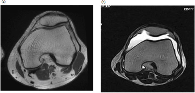 | |
| Fig. 1:(a, b) | (a) Normal Axial view of knee joint and (b) Effusion in knee joint |
 | |
| Fig. 2: | Block diagram for proposed methodology for knee effusion |
Before usage of the filter, it is expected that the user knows the spectral properties of the initial signal and noise. Spectral properties are just like the control functions for both the initial signal and noise. The resultant signal requires is as near to the original signal. Signal and noise are both stochastic procedures with known spectral properties. The point of the method is to have minimum mean square error. That is the distinction between the first signal and the new signal should be as less as could reasonably expected. The Weiner filter is ideal in terms of the mean square error. In other words it minimizes the general mean square error within the process of inverse filtering and noise smoothening. The Weiner filter may be a direct estimation of the original picture. The methodology depends on the stochastic system. The symmetry rule infers that the Weiner filter in Fourier space can be defined as:
| (1) |
Where:
| F | = | The Fourier transform of original picture |
| H | = | The blurring function |
| H(u, v) | = | The received signal |
| G(u, v) | = | The restored image |
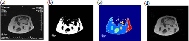 | |
| Fig. 3(a-d): | Watershed Segmentation of knee joint in axial view (a) Given image (b), Thresholded image (c) watershed region extraction and (d) Segmented image using watershed segmentation |
Image segmentation: Image segmentation is a basic procedure for most consequent picture investigation assignments. In specific numerous of the existing strategies for picture portrayal and acknowledgement, picture visualization and object based picture compression profoundly depend on the division results. The common division includes the apportioning of a given picture into a number of homogenous sections such that the union of any two neighboring sections yields a heterogeneous section. On the other hand division can be considered as a pixel naming procedure as in all pixels that have a place with the equivalent homogenous area is appointed a similar mark. There are a few different ways to characterize homogeneity of a region based on the specific objective of the division procedure.
Feature extraction
Watershed segmentation: The present techniques for picture fundamentally utilize two thoughts. One of them is finding the form of objects in the picture. The other is gathering focuses with similar characteristics, so that, the object of interest is completely recreated. The issue of contour distinguishing proof may be illuminated with the utilization of the watershed administrator which is the primarily morphological segmentation division tool known as water line. An instinctive thought of the watershed idea might be formed considering the gray levels picture as a topographic surface and expecting that gapes have been punctured in each territorial least of the surface. The surface is then gradually emerged into water. Beginning from the base at the most minimal height, the water will progressively flood the maintenance basins of the picture. In expansion, dams are raised at the places, where the water coming from the unique essentials would rise. Towards the part of this flooding strategy, each least is encompassed by dams portraying its associated retention basin. The entire arrangement of dams compare to the watersheds. They provide us with portion of an input picture into its distinctive basins[7]. Watershed related to the regional minimums set M = Ui∈R mi of an image S may be characterized as the union complement of all maintenance basins Cf (mi) and can be defined by the following equation as:
| (2) |
Watershed segmentation is a powerful scientific morphological tool for the picture division. It is most used in medical image processing and computer vision[8]. Watershed implies the edge that partitions ranges drained by distinctive waterway frameworks. In the event that picture is seen as topographical scene, the watershed lines decide limits which isolate picture regions. The watershed change registers catchments basins and ridge lines where catchments basins comparing picture areas and ridge lines identifying with area limits. Watershed segmentation dependent on watershed change have fundamentally two classes[21]. The first class contains the flooding based watershed segmentation whereas the second class contains rain falling watershed algorithms. Numerous algorithms have been proposed in the two classes but associated components based watershed algorithm appears exceptionally great execution compared to all others. It comes under the rain falling based watershed algorithm procedure. It gives exceptionally great division results and meets the criteria of less computationally complexity for hardware execution.
Watershed transform: It is an effective mathematical morphological tool for the picture division. Watershed algorithm involves three essential steps gradient of the image flooding segmentation. In the initial step, the slope of the picture is calculated[9]. It demonstrates the directional change in the color of the picture. The next step includes the development of the catchment basin and flooding[10]. In this step on the off chance we consider the picture a scene picture at that point the gap is punctured there, where the power is exceptionally low. Moreover where the gap is punched that is called as the catchment basin. After that the flooding procedure begins when that topographic relief is overwhelmed with water, the separate lines of the areas falling over the locales structure of the watersheds. Naturally a drop of water falling on a topographic relief steers towards the closest minimum. The closest minimum is that minimum which lies toward the part of the steepest plunge. These minima are the neighborhood minima. The water topped of at the beginning nearby minima and focuses where water coming from various basins would meet and dams will be worked. The third step prompts the development of dams[11]. In light of the fact that towards the part of the arrangement procedure dams come into record and these dams shapes the unbending watershed lines.
 |
|
| Fig. 4: | 2-D complex gabor filter with 32 coefficients (4 frequencies and 8 orientations) |
These dams maintain a strategic distance from an occasion which comes during the flooding when at least two floods coming from various minima may consolidate. These dams characterize the watershed of the capacity of a picture. This isolates the various catchments basins (Fig. 3).
D gabor filter: Gabor filter is a linear filter utilized for the detection of an edge. The frequency and direction portrayals of Gabor filters are like those of human visual framework and they have been observed to be especially fitting for surface portrayal and separation. In the spatial domain a 2D Gabor filter is a Gaussian kernel function adjusted by a sinusoidal plane wave. The Gabor filters are self-comparative; all filters can be created from one mother wavelet by dilation and rotation. The 2D complex Gabor filter is particularly useful for removing a set of characteristics in multiple orientations and frequencies of an image[12]. Complex 2D Gabor filtering for all pixels for an image however; causes an expanse costs. With the Gabor core defined in a specific orientation and frequency, filtering is done by moving a reference pixel by pixel. The core complex of Gabor hinders fast filtering in context similar to filters with edge recognition[13].
To speed up 2-D complex Gabor filter, a few efforts have been made for occurrence by making utilize of FFT (Fast Fourier Transform), IIR (Infinite Impulsive Response) filters of Finite Impulsive Response (FIR) filters. It was appeared[14] that Gabor filter for 1-D signal of N tests can be performed with the same complexity as of the FFT O (NlogN). In[15] distinct FIR filters are connected to perform quick 2D complex Gabor filtering by exploiting special relationship between the Gabor parameter in a multi-resolution pyramids.Its impulsive reaction is characterized by a harmonic function motivated by a Gaussian function. In light of the multiplication convolution property, the Fourier change of a Gabor filters motivation reaction is the convolution of the Fourier change of the harmonic function and the Fourier change of the Gaussian function. The filter contains a genuine and an imaginary component speaking to orthogonal headings. The two components may be shaped into a complex number or utilized separately. A 2D Gabor filter is defined as:
 | (3) |
The spread of the Gaussian work in x and y directions have been signified by σx and σy symbols separately. The Gabor channel bank is connected on the pictures considering the focus recurrence to mean the direction of the filters. In the recurrence area the Gabor filter depends on the two dimensional 2D recurrence and direction. In this study we take over eight diverse direction and recurrence situations and a Gabor space is made by convolving these channels with the test pictures. The recurrence response of the filter is given by the equation:
| (4) |
Where, a[(u-u0)2 σ2x] &b = [(v-v0)2 σ2 y]. In this way, Gabor function can be thought as being a Gaussian work moved in recurrence (Fig. 4). The middle recurrence of the filter is indicated by the recurrence of the sine/cosine wave and the bandwidth of the channel is balanced by the width of the Gaussian. A 2D Gabor filter over on image space (x, y) as:
 | (5) |
Where:
| X0 and y0 | = | The Positions in the image |
| α, β | = | The effective width and length |
| u0, v0 | = | Specific modulation which has spatial frequency |
 | |
| Fig. 5: | Random rorest |
 | |
| Fig. 6: | Back propagation neural network |
Classification
Random forest: Random forest is a machine learning that is progressively being utilized for classification and regression consists of an ensemble of independent decision tress. It is a group of model which implies that it utilizes the outcomes from a wide range of models to ascertain a reaction. In most cases the result from an ensemble model will be superior to the result from ant one of the personal model. Within the case of Random forest a few choice tress are made and the response is calculated based on the result of all the choice tress. It consists of a number of trees where each tree is developed employing a shape of arrangement. The leaf nodes of each tree are labelled by gauges of the ensuing dispersion among the sorts of pictures. Each node inside the tree follows a test that separates the space superior of information to classify. An image can be classified by sending it down through each tree and accumulating to come to leaf distributions. Randomness can be infused at two cases amid in training: In sub-sampling of training information, so that, each tree is developed employing a distinctive subset and when selecting the nose testing (Fig. 5 and 6):
The trees are binary and built from in a top-down way. Binary tests at every node can be picked in one of the two different ways randomly by combining the yield of different randomized trees into a single classifier. They have been illustrated to deliver lower test errors than conventional decision trees[12]. The best here is measured by the data gain caused by dividing the set of Q illustrations into two subsets Qi, concurring the given test:
 | (6) |
E(q) is the entropy with pj the extent of illustrations in q having a place with class j and |.| the size of the set. The procedure of choosing a test is repeated for each non-terminal node utilizing as it were the preparing illustrations falling in that node. The recursion is halted when the node gets excessively few models. If we assume that T is the size of all trees, C is the set of all classes and L is the set of all clears out for a given tree. Amid the preparing stage the back probabilities (Pt, 1(Y(I) = c) for each class c∈Cat each leaf node l∈L are found for each tree t∈T. These probabilities are determined as the proportion of the quantity of pictures I of class c that arrive at l to the absolute number of pictures that arrive at l. Y(I) is the class name c for picture I.
Classification: The image for testing purpose is passed down each random tree until it comes to a leaf node. All the back probabilities are at that point found the middle value of the arg max is taken as the classification for the input picture. It is a decision tree gathering classifier with each tree developed utilizing a few sort of randomization. Random forests have a capacity for preparing huge amount of information with high preparing spaces in view of a choice tree. The structure of each tree in the random forest is twofold and is made in a top-down way as shown in Fig. 5. In this research we consider binary trees with their structure and choice nodes learned discriminatively as pursues. Beginning from the root given the named preparing data, the function t and threshold λ which maximize the data pick up are found. Then preparing continues down to the children nodes.
In the preparing technique the random forest begins by picking an arbitrary subset I from the neighborhood of Gabor filter preparing information. At the node n the preparing information In is iteratively split into left and right subsets II and Ir by utilizing the limit t and split function F(vi) for the feature vector v using Eq. 5. The threshold t is arbitrarily picked by the split function F(vi) in the range t∈(min F(vi) max F(vi)):
| (7) |
| (8) |
At that point a few candidates are haphazardly made by the split function at the split node. Among those, the candidate that amplifies the data increase about the relating node is chosen. The data gain ΔE is effectively determined by entropy estimation given by the equation:
 | (9) |
There are two conditions that can conclude the iterative training. The primary condition happens in case there is no more data increase conceivable. The subsequent condition happens if the preparing procedure arrives at a leaf node that is at the greatest depth of the tree. Thus a leaf node has a posterior likelihood and the class ci disseminations P(c/n) and assessed experimentally as a histogram of class ci of the preparing models that arrived at node n. The test picture is utilized as input to the prepared random forest. The ultimate class distribution is produced by gathering of each dispersion of all trees L = (l1, l2, l3, ..., lr) by utilizing the following equation:
| (10) |
Where, T is the number of trees and we select ci as the last class of an input picture if P(ci/L) has the most extreme values.
Multi-Layer BPNN (Back Propagation Neural Network): BPNN (Back Propagation Neural Network) is a method for preparing multi-layer ANN (Artificial Neural Network)[17]. It is a multi-layer forward system utilizing to expand gradient descent based delta learning rule known as back propagation. It gives a computationally efficient strategy for changing the loads in a feed forward system with differentiable function work units to get familiar with a training set of input yield being a gradient descent strategy; it minimizes the full squared error of the yield computed by the system. The system is prepared by supervised learning strategy. The basic structure of the BPNN incorporates one input layer at least one hidden layer followed by the output layer. Neural system works by modifying the weight values during preparing, so as to lessen the error between the real and desired output design[18]. The goal of this system is to prepare the network to achieve an adjustment between the capacity to react accurately to the input designs that are utilized for training and the ability to give great reaction to the input that are similar (Fig. 6).
It has three kinds of layers Input layer, Hidden layer and output layer. Hidden layer does middle computation before guiding the input to output layer. Moreover back propagation can be considered as a generalization of delta rule. At that point when the back propagation system is cycled an input pattern is proliferated forward to the output units through the interceding input to hidden layer and then hidden to output weights. It consists of numerous layers of computational units, normally interconnected in a feed forward manner. Each neuron in one layer has coordinated associations with the neurons of the subsequent layer. In numerous applications, the units of these systems apply a sigmoid function as an enactment work function. All inclusive estimation hypothesis for neural system states that each continuous function that maps interims of genuine numbers to a few output interims of genuine numbers can be approximated discretionarily intently by a multi-layer preceptor with only one hidden layer.
This outcome holds just for confined class of activation functions. Multi-layer system[15] utilizes an assortment of learning methods, the most well-known back propagation. In this the output values are compared with the proper reply to compute the estimation of a few predefined error functions. By different systems, the error is then encouraged back through the system. Utilizing this data, the algorithm adjust the weight of each association in arrange, so as to decrease the value of the error function just barely. After repeating this procedure for an adequately expansive number of preparing cycles, the system will more often than not to meet to a few states, where the error of the calculation is little.
Implementation of BPNN: BPNN algorithm compromises of the following steps. Each input is increased by a weight either inhibit the input or energize the input. The weighted sum of the inputs at that point is calculated first, it computes the entire weighted input by using the following equation:
| (11) |
Where:
| Yi | = | The activation level of the jth unit within the previous layer |
| Wji | = | The weight of the association between the ith and jth unit. At that point the weighted |
| xj | = | Passed through a sigmoid work that would scale the outcome in between 0 and 1 |
Furthermore, the unit computes the activation utilizing a few function of the overall weighted input. We use the sigmoid function as:
 | (12) |
When the output is determined, it is contrasted with the required output and the overall error is calculated. When the activities of all the output units had been resolved, the system figure out the error E, which is characterized by the equation.
 | (13) |
yi is the activation level of the ith unit within the top layer and dj is the specified output of the ith unit. It calculates how quick the error changes as the action of an output unit are changed. This error EA is the distinction between the genuine and desired output:
| (14) |
Calculates how quick the error changes as the whole input received by an output unit is changed. This amount (EI) is the appropriate response from stage 1 duplicated by the rate at which the yield of an unit change as it add up to input is changed:
 | (15) |
Calculates how quick the error changes as a weight on the connection into an output unit are changed. This amount EW is the reply from step 2 increased by the action level of the unit from which the association radiates:
 | (16) |
It calculates how quick the error change as the action of a unit in the previous layer is changed. This vital step permits back propagation to be connected to multi-layer systems. Whenever the moment of a unit in the previous layer transforms, it influences the activities of all the output units to which it is associated. To calculate the impact on the error, we include all these different impacts on outputs units. But each impact is easy to compute. It is the appropriate response in step 2 increased by the weight on the association with that output unit. By utilizing step 2 and step 4 we can change over the EA’s of one layer of units into EA’s for the previous layer. This methodology can be rehashed to get the EA’s for the same number of layers as wanted. When we know the EA of a unit we can utilize step 2 and 3 to compute the EW’s on its approaching association:
 | (17) |
Adaboost SVM: Adaboost with SVM based component classifier is generally considered to break the Boosting rule for the trouble in preparing of SVM and have lop-sidedness between the difference and exactness over fundamental SVM classifiers. The Adaboost classifier within the paper trains SVM as base classifier with changing kernel function parameter value which continuously diminishes the changes of weight value in training test. To affirm the legitimacy of the classifier, the classifier is tried on human subjects to classify the right and left knee effusion imagery tasks. The running time for preparing algorithms for SVM can be diminished, if just a barely any preparing illustrations are included with the real calculations. This truth can be exploited by Adaboost, if at every cycle most of the weight within the distribution passed to the powerless learner is allocated to many information points. The calculation time can be diminished as pursues. One of the off chances if the complexity of the original preparing calculations is bounded A by mx with A∈R at that point training with a fraction vm is bounded by A(vm)x. Hence, preparing q speculations is bounded by A(vm)x. Then if x>v1, 0>v>1 and q≤1/v:
 | (18) |
The classification execution of Adaboost SVM is affected by its parameters. For SVM-RBF, the parameters are Gaussian width σ and regularization parameter C. SVM-RBF classifiers performance generally depends on the σ value in case a generally appropriate C is choosen[19]. For a given C, the performance of SVM-RBF can be changed by essentially altering the value of σ. Expanding the value often decreases the complexity of learner model and bringing down the classification execution and vice-versa. So when the SVM-RBF is utilized as powerless classifier for Adaboost, a moderately huge value is liked, which brings a SVM-RBF with moderately powerless learn capacity[20].
The Adaboost calculation makes a set of destitute learners by keeping up a collection of weights over training information and alters then after each powerless learning cycle adaptively. The weights of the training samples which are misclassified by current frail learner will be expanded while the loads of the tests which are accurately grouped will be diminished. One of the fundamental thought of Adaboost algorithm is to keep up a circulation over the preparing set. The weight of this dispersion on preparing model i on round t is signified Dt(i). At first, all loads are instated similarly, however on each round; the loads of erroneously classified cases are increased, so that, the frail learner is forced to center on the difficult illustrations within the exchanging set. The feeble learner responsibility is to discover a frail theory ht:x{-1, +1} suitable for the appropriation (D)t. Given: (x1, y1), ... , (xn, yn) where x1∈X, y1∈Y = {-1, +1}. When applying Boosting strategy to solid component classifier, these component classifiers must be suitable depilated in arrange to advantage from boosting. Consequently, if SVM-RBF is utilized as component classifier in Adaboost, a generally expansive value which corresponds to a SVM-RBF with generally powerless learning ability is favoured. In the proposed Adaboost SVM, without loss of simplification, the re-weighting strategy is used to refresh the loads of preparing tests. Adaboost can be depicted as pursues.
At first, a huge worth is set to σ, comparing to a SVM-RBF classifier with exceptionally feeble learning capacity. At that point, SVM-RBF with this σ is prepared, however many cycles as conceivable under the circumstances as long as beyond more than half exactness can be gotten. Otherwise this σ worth is diminished marginally to expand the learning capacity of SVM-RBF to enable it to accomplish the more than half accuracy. By diminishing the σ value marginally, this avoids the new SVM-RBF from being solid for the current weighted preparing tests and hence decently exact SVM-RBF segment classifiers are acquired. The reason why moderately exact SVM-RBF component classifiers are favoured lies in the way that these classifiers regularly have bigger assorted variety than those segment classifiers which are exceptionally exact. These bigger assorted varities may prompt a superior speculations execution of Adaboost. This procedure proceeds until the σ is diminished to the given insignificant value.
RESULTS AND DISCUSSION
Experiments and results: This experimental study was taken on 203 patients. MRI images have been collected from different medical institutes. Most of the image size was 350×350 and some of the image size was 630×630. To maintain the uniformity, the image is resized into 250×250. From the obtained images, some of the images are already availing in grayscale mode and the rest of the images which was not available in the grayscale have been converted to the gray scale image. In the pre-processing mode, wiener filter is applied to remove the noise. To extract the region of interest, watershed segmentation is applied. Using the gradient magnitude as the segmentation function, first it splits the foreground objects. Image gradients can be used to extract information from images. Each pixel of a gradient image measures the change in intensity of the same point in the original image, in a given direction. To get the full range of direction, gradient images in the x and y directions are computed.
With the help of watershed transform segmentation function, unwanted background information such as text and other information had been removed from the knee joint MRI image. The watershed transform is often applied to this problem. The watershed transform finds “catchment basins” and “watershed ridge lines” in an image by treating it as a surface where light pixels are high and dark pixels are low. Segmentation using the watershed transforms works well if one can identify, or “mark” foreground objects and background locations. Binary Marker-controlled watershed segmentation follows this basic procedure:
| • | Compute the dark regions; it helps us to identify the segmentation regions. Apply the binary mask |
| • | To calculate the foreground, connect the blobs of pixels within each of the objects |
| • | Background markers will be considering the pixels that are not part of any object |
| • | Remove the background blobs |
| • | Compute the watershed transform of the modified segmentation function |
After extracting region of interest, Gabor features are extracted from the image. Gabor filters have been used in many applications such as texture segmentation, target detection, fractal dimension management, document analysis, edge detection, retina identification, image coding and image representation[24]. First step of Gabor feature extraction is generating custom-sized Gabor filter bank. It creates a u by v cell array, whose elements are m by n matrices, each matrix being a 2-D Gabor filter. The second step is to extract the Gabor features of an input image. It creates a column vector, consisting of the Gabor features of the input image. The feature vectors are normalized to zero mean and unit variance.
Classification is final step to produce the result. In classification, three classifiers have been utilized namely Random Forest, BPNN and Boosting SVM are experimented separately. In Random Forest, the root node we chose r = 2, a very small number, to reduce the correlation between the resulting trees. For all other nodes, we used r = 100 D, where D is the depth of the node. Inclassification trees, the splitting decision is based on the following methods:
| • | Gini index it’s a measure of node purity. If theGini index takes on a smaller value, it suggests that the node is pure. For a split to take place, the Gini index for a child node should be less than that for the parent node |
| • | Entropy-entropy is a measure of node impurity. For a binary class (a, b), the formula to calculate it isshown below. Entropy is maximumat p = 0.5. For p(X = a) = 0.5 or p(X = b) = 0.5 means, a new observation has a 50-50% chance of getting classified in either classes. The entropy is minimum when the probability is 0 or 1: |
| (19) |
When choosing a binary test randomness is injected into the training set per tree: one third of the training images per category are randomly selected and used to determine the node tests by the entropy criterion and the remaining training images are used to estimate the posterior probabilities in the terminal nodes. This heuristic involves randomizing over both tests and training data. When using the simpler approach, trees are grown by randomly selecting n and b without measuring the gain of each test and all the training images are used to estimate the posterior probabilities.
The classification process is done with Boosting SVM. Normally, AdaBoost classifiers are having less tuning parameters compared to SVM and SVM is not affected by the noise sensitivity. This tuning parameter is mainly used for improving the performance of classifiers. Here, the kernel function is used to improve the performance of the SVM. This methodology gives the RBF kernel for mapping the data into high dimensional space. The RBF kernel function is a best measurement for finding the similarity between normal and abnormal images. This similarity will be calculated using the texture feature and the corners of the shape feature.
Back-propagation is the essence of neural net training. It is the method of fine-tuning for the weights of a neural net based on the error rate obtained in the previous epoch (i.e., iteration). Proper tuning of the weights allows you to reduce error rates and to make the model reliable by increasing its generalization. The randomly obtained initial synaptic weight of the neural network covers a range between -0.5 and 0.5. Best method of testing a neural network is to test a software application if all the coverage conditions are satisfied. It iteratively learns a set of weights for prediction of class label tuples. The predicted output is compared with target value to check the error. This algorithm is type of supervised learning and used in feed forward neural network to train the network. The results of these three classifiers were compared. Those results are listed out in Table 1-6.
The average accuracy rate 88.92% is calculated from adaboost with SVM, 90.94% is calculated from BPNN and 92.12% is calculated from Random Forest. We report the advancement and approval of a mechanized Table 1: Results obtained from random forest classifier framework for quantitative volume assurance of knee joint effusion in MRI pictures.
| Table 2: | Classification metric for random forest |
 |
|
| Table 3: | Results obtained from Adaboost with SVM |
 |
|
| Table 4: | Classification metric for Adaboost with SVM |
 |
|
| Table 5: | Results obtained from back propagation neural network |
 |
|
| Table 6: | Classification Metric for BPNN |
 |
|
Two conventions intended to approve the created innovation, one utilizing adjusted phantoms and another going for examination with a manual strategy, indicated magnificent reproducible outcomes. Further, correlation between the joint effusion volume obtained by MRI pursued by evaluation with the created computerized framework and the immediate desire performed on knee OA patients additionally showed a superb connection.The MRI convention incorporated a T1-and a T2-weighted pivotal arrangement. The decision of axial arrangements came about from the need to lessen incomplete volume impact on the division of the joint effusion. In view of the fundamental direction of the synovial pocket along the bones, the other obtaining planes, sagittal and coronal, would have delivered progressively fractional volume. In spite of the fact that the T2 grouping improved the joint emission signal, the other liquid like tissues, for example, blood, a few hyaline cartilage, and bone marrow sores, too showed up brilliant. Subsequently, the utilization of intensity property just would not be adequate to segment the joint effusion dependably. In this way, the bone was utilized as an anatomic reference for 3D item filtering. T2 arrangement does not give a maximal differentiated signal for the bone, the T1 grouping was utilized for the division of the femur and tibia, as they show up more clear and progressively homogeneous on the picture.
CONCLUSION
The effusion of knee joint is a typical finding in OA patients and might be identified with the action of the disease. Accordingly non-invasive completely computerized evaluation of joint effusion volume in the knee would be an important apparatus for indicative, development and clinical investigation. The detailed automatic framework for joint effusion volume evaluation approved by outer methods, manual MRI evaluation and direct goal was demonstrated to be exact and precise, in expansion to preventing intra and inter-observer varities. The responsiveness to alter of automatic assessment of joint effusion ought to be additionally tried in al longitudinal examination in perspective on its future application in clinical; research. In spite of an assessment of clinical tests to evaluate joint effusion in knee OA, the larger part of unstandardized test had generally low intraand inter-observer unwavering quality. Unwavering quality and demonstrative accuracy seems to be made with involvement. Compared to indidual tests employing a combination of tests for effusion seem to improve affectability. There is inadequately proof to suggest a specific test in clinical practice. Clinical involvement and effusion profundity may influence the accuracy of clinical examination in identifying knee effusion in patients with knee osteoarthritis. MRI may help clinicians in accomplishing a more precise determination, superior therapeutic decision, as well as objective measure in clinical outcomes. In this work we have utilized two feature extraction processes namely Watershed segmentation and 2-D Gabor Filter were computed. For classification purpose, Random Forest, Multi-layer BPNN and Adaboost SVM are employed. When compared to the classification result one with each other, Random Forest gives the best accuracy than other two classifiers for this work. The proposed method has achieved the maximum classification accuracy rate of 92.12%. In future work, the aim is to enhance segmentation and classification rate by using still better methods for pre-processing, segmentation, feature extraction and classification. In conclusion the knee joint effusion was not static in more in older adults. It was prescient of, but not predicted by other structural variations from the normal recommended a potential part in early knee OA changes.